In your learning path, you might notice than learning by doing things is a lot more of fun and you learn better and faster. Especially, with Data Science、there're a lot of resources available out there, and it might be frustrating spending your time reading books over and over. You can put into practice your knowledges by building a data science side project, but it might not be always suitable for beginners. That's why Kaggle is for. Kaggle is a website hosting competitions for you to work with real-world datasets by creating predictive models. It allows you to use whatever tools or language you want to build your models. There're lots of competition out there, in this post I'll show how to build a machine learning predictive model to predict the type of tree for the Forest Cover Type Prediction, which is a good competition to begin with and deals with a muti-class classification.

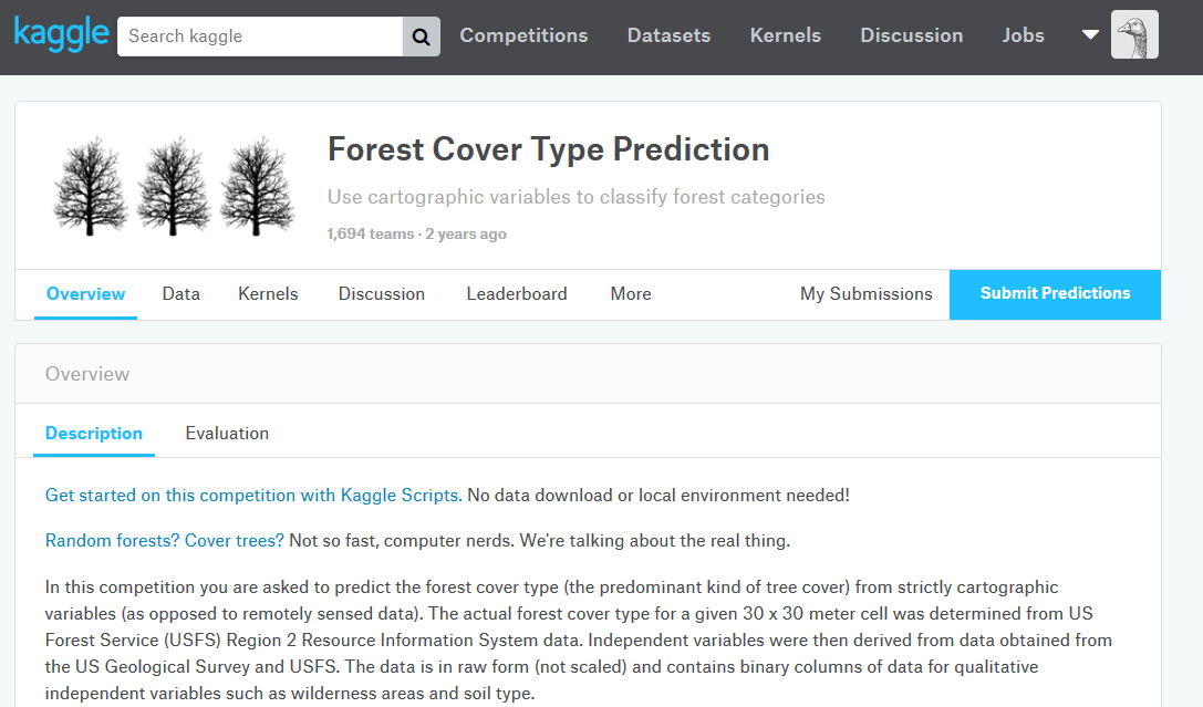
Now, start with reading the competition description and downloading the dataset in the Data tab, here you got the training dataset, the testing dataset and the submission sample file (all in .csv file). Read carefully the dataset description and the content of the dataset. Generally, for a supervised model, the training dataset provide the label where the testing dataset doesn't. It's up to you to predict these labels after training your model on the training dataset. For this study, I'm using Jupter Notebook and  Python libraries such as Pandas for processing and cleaning the data, Scikit-learn for creating the machine learning model and Seaborn/Matplotlib for the plot/graph visualization.

For my full Jupyter Notebook workflow, check out my GitHub link.

Processing the data

We start by important the training and testing dataset into a pandas dataframe and check out the variables of the file.

import numpy as np
import pandas as pd
import matplotlib.pyplot as plt
import seaborn as sns
%matplotlib inline

train = pd.read_csv('data/forest_train.csv')
test = pd.read_csv('data/forest_test.csv')

train.head()

And here's how the training dataset looks like:

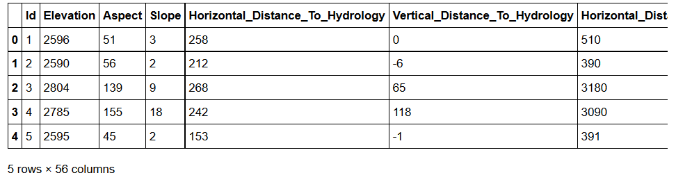
Now, let's check whether or not the dataset contains any missing values (no missing, null or NaN values in this case).

train.isnull().sum()
>>> 0

We start with seeing the distribution of the attribute Elevation for each tree by plotting a histogram.

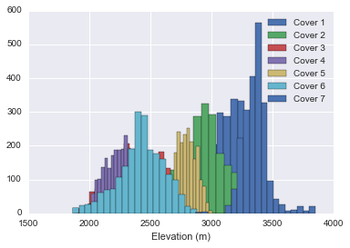
Only with this plot, we can suppose  that the Elevation feature has an important weight, since we can already distinguish the type 3, 4 and 7 with only this attribute.

We can then check for the Hillshade attribute by plotting a scatter plot.

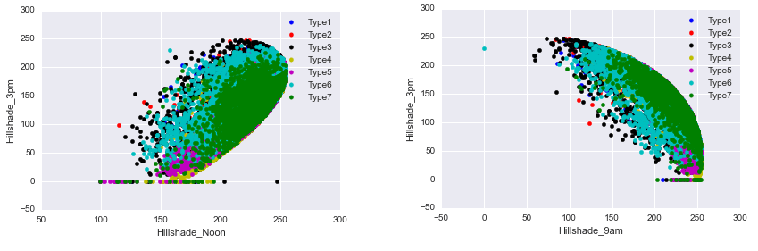
Several values are equal to zero for the Hillshade_3am., and we can then suppose that these are the missing values and can replace them with the mean of the attribute.

Features engineering

Often, the features of a dataset cannot be used as it was provided, we have to create a new meaningful feature based on those provided by the raw dataset. For example, we can combine the two features Horizontal_Distance_To_Hydrology and Vertical_Distance_To_Hydrology into a single dist_to_water feature which represents the euclidean distance to the water for each tree.

dist_to_water = train.loc[:, ['Horizontal_Distance_To_Hydrology', 'Vertical_Distance_To_Hydrology']].apply(lambda x: np.sqrt(x[0]**2 + x[1]**2), axis=1)
dist_to_water_test = test.loc[:, ['Horizontal_Distance_To_Hydrology', 'Vertical_Distance_To_Hydrology']].apply(lambda x: np.sqrt(x[0]**2 + x[1]**2), axis=1)

dist_to_water = pd.DataFrame(dist_to_water, columns=['dist_to_water'])
dist_to_water_test = pd.DataFrame(dist_to_water_test, columns=['dist_to_water_test'])

train = pd.concat([train, dist_to_water], axis=1)
test = pd.concat([test, dist_to_water_test], axis=1)

train[['Cover_Type', 'dist_to_water']].groupby('Cover_Type').mean().plot(kind='bar', title='Distance to water for each type')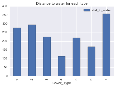

Categorizing features

In this dataset, there are 4 columns for the Wilderness_Area attribute and 40 columns for the Soil_Type. These columns are binary, e.g., their content are either 1 (presence of the given attribute) or 0 (absence). For example, a given tree has 1 in the colunm Wilderness_Area3 and 1 in the Soil_Type26 means that this tree belongs to the wilderness area 3 and has the 26th soil type.

Instead of having plenty of binary columns, I combined these attributes into 2 categoical columns, which has possible value of 1 to 4 for the Wilderness_Area feature, and 1 to 40 for the Soil_Type feature. Here's how it can be done with Pandas :

# categorize the 4 columns of Wilderness_Area into 1 single column
def categorize(df, cols_name):
    for k in range(df.shape[1]):
        df[cols_name+str(k+1)] = df.loc[:, cols_name+str(k+1)].map({1:k+1, 0:0})
    return df

wilderness = train.loc[:, 'Wilderness_Area1': 'Wilderness_Area4']
wilderness = categorize(wilderness, 'Wilderness_Area')
wilderness = wilderness.sum(axis=1).astype('category')
train = pd.concat([train, wilderness], axis=1)

wilderness_test = test.loc[:, 'Wilderness_Area1': 'Wilderness_Area4']
wilderness_test = categorize(wilderness_test, 'Wilderness_Area')
wilderness_test = wilderness_test.sum(axis=1).astype('category')
test = pd.concat([test, wilderness_test], axis=1)



# categorize the 40 columns of Soil_Type into 1 single column
soil = train.loc[:, 'Soil_Type1': 'Soil_Type40']
soil = categorize(soil, 'Soil_Type')
soil = soil.sum(axis=1).astype('category')
soil = pd.DataFrame(soil, columns=['soil'])
train = pd.concat([train, soil], axis=1)

soil_test = test.loc[:, 'Soil_Type1': 'Soil_Type40']
soil_test = categorize(soil_test, 'Soil_Type')
soil_test = soil_test.sum(axis=1).astype('category')
soil_test = pd.DataFrame(soil_test, columns=['soil_test'])
test = pd.concat([test, soil_test], axis=1)

Building the predictive model

The last step before the submission is to build a predictive model which will be trained on the cleaned training dataset. Then, I used this predictive model to predict the Cover_Type of each tree in the testing dataset using scitkit-learn.

Here I used two machine learning algorithms, k-Nearest Neighbors (KNN) and Random Forest to predict the type of each tree in the testing dataset. For the KNN, here's the code :

from sklearn.neighbors import KNeighborsClassifier

x_train = train[['Elevation', 'Aspect', 'Slope', 'Horizontal_Distance_To_Roadways', 'Horizontal_Distance_To_Fire_Points', 'dist_to_water', 'Hillshade_Noon', 'Hillshade_3pm', 'Hillshade_9am', 'soil']]
y_train = train.Cover_Type
x_test = test[['Elevation', 'Aspect', 'Slope', 'Horizontal_Distance_To_Roadways', 'Horizontal_Distance_To_Fire_Points', 'dist_to_water_test', 'Hillshade_Noon', 'Hillshade_3pm', 'Hillshade_9am', 'soil_test']]

knn = KNeighborsClassifier()
knn.fit(x_train, y_train)
y_test = knn.predict(x_test)

submission003 = OrderedDict([('Id', test.Id), ('Cover_Type', y_test)])
submission003 = pd.DataFrame.from_dict(submission003)
submission003.to_csv('submission/forest_submission003.csv', index=False)

After predicting on the testing dataset, I convert the result into a csv file to submit on Kaggle. This submission using KNN got me a score of 0.63445, which means that 63% of the predictions are correct.

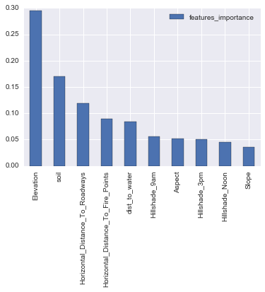
With the same process, I trained and predicted using the Random Forest algorithm and I got a score of  0.71449. This algorithm also allow to see the importance of each feature in the dataset, regarding the prediction. We can see as expected that the Elevation attribute has a great importance as shown in the plot below:

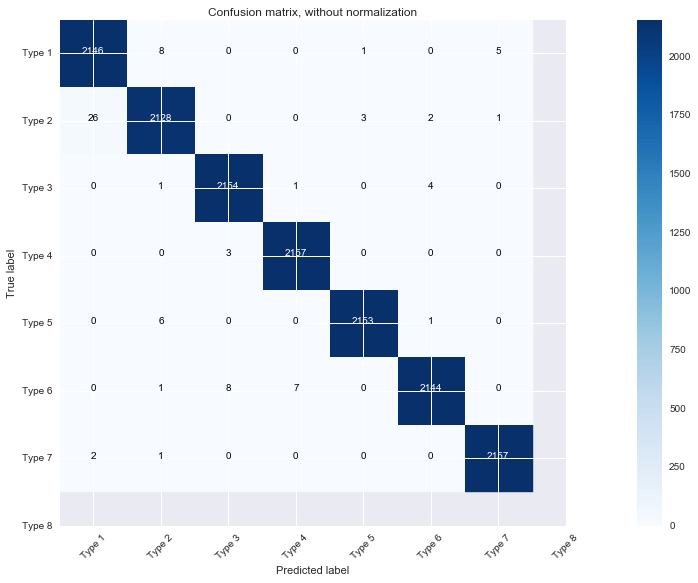
I also plot the confusion matrix on the training dataset, and the result shows that the most difficult to predict types, are the types 1 and 2.

This is my first Kaggle competition, and I think, to begin with, it's a good dataset to explore in order to get used to all the tools and methods available for data science. There are similar ones for beginner such as :

• Titanic: Machine Learning for Disaster for Binary Classification
• Bike Sharing Demand for Regression with temporal component
• Random Acts of Pizza for Binary Classification with text data

To see the full Jupyter Notebook code, please check out my GitHub repository.